When Data Falls Silent: Diagnosing Missing Data Mechanisms

Stanis B.

April 15, 2026 · 7 min read

Every real dataset has holes. A column full of blanks, a timestamp that simply never arrived, a field the respondent left empty — on the surface they all look the same. In practice they are not. The reason a value is missing is as important as the value itself, and conflating different reasons leads to models that are quietly, confidently wrong. A patient cohort where sicker people drop out of a trial is a different problem than a sensor that randomly powers off. Imputing both the same way is the kind of mistake that passes cross-validation and fails in production.

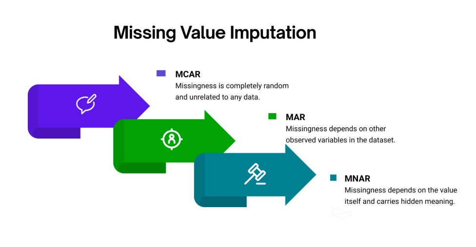
The field has three named mechanisms for why values go missing. MCAR — missing completely at random — is the benign case: the absence of a data point has nothing to do with anything measured or unmeasured. MAR — missing at random — is more subtle: the probability of missingness depends on other observed columns, but not on the value that is actually missing. MNAR — missing not at random — is the hard case: the value is absent precisely because of what it would have been. An understanding of which regime you are in changes everything that follows — which tests to run, which imputer to trust, and how much uncertainty to carry forward into your downstream model.

What follows is a working guide to diagnosing and handling all three, with Python code you can adapt to real pipelines.

MCAR — the benign blank

"A sensor randomly drops a packet. A survey respondent accidentally skips a page. The phone dies mid-form. The value is gone for reasons entirely unrelated to the data itself."

MCAR is the statistician's dream and the practitioner's most overused assumption. When data is truly missing completely at random, the rows with missing values are an unbiased random sample of all rows. You can delete them without introducing systematic error. You can fill them with the column mean without distorting the distribution in any directional way. The danger is not in the technique — it is in the diagnosis. Many analysts assume MCAR because it is convenient, not because they have tested it.

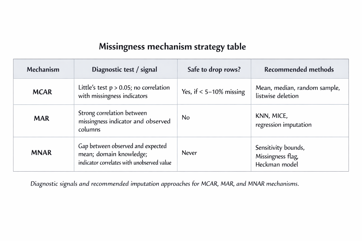
Little's MCAR test gives you a formal chi-squared statistic. A high p-value (conventionally above 0.05) provides evidence you cannot reject the MCAR hypothesis. It is not proof — it is a failure to disprove. Combine it with a visual missingness heatmap and an examination of whether missingness correlates with any observed column before you commit.

MCAR: Use cases

MCAR most commonly appears in IoT sensor streams with random dropout, large paper surveys with accidental skips, and automated data collection pipelines with transient network failures. It is far rarer in human-generated survey data on sensitive topics, where structured avoidance tends to dominate.

MCAR: Techniques

For MCAR, your choices are: mean or median imputation (fast, preserves column-level statistics), random sample imputation (preserves the full empirical distribution), or listwise deletion (removes the row entirely). The last option is only defensible when the percentage of missing rows is small — under five percent is a rough rule of thumb — and the dataset is large enough to absorb the loss..

python

1import pandas as pd
2import numpy as np
3from scipy.stats import chi2
4
5np.random.seed(42)
6n = 400
7
8df = pd.DataFrame({
9    'age': np.random.randint(20, 65, n).astype(float),
10    'income': np.random.randint(25000, 95000, n).astype(float),
11    'score': np.random.randint(300, 850, n).astype(float),
12    'tenure': np.random.randint(0, 30, n).astype(float)
13})
14
15# Introduce 15% MCAR — purely random mask
16random_mask = np.random.rand(*df.shape) < 0.15
17df[random_mask] = np.nan
18
19print("Missing counts per column:")
20print(df.isnull().sum())
21
22total_missing = df.isnull().sum().sum()
23pct_missing = df.isnull().mean().mean()
24
25print(
26    f"\nTotal missing: {total_missing} of {df.size} cells "
27    f"({pct_missing:.1%})"
28)
29
30
31def littles_mcar_test(data: pd.DataFrame):
32    """
33    Approximate Little's MCAR test.
34    H0: data is MCAR.
35    High p-value → insufficient evidence to reject MCAR.
36    """
37    d = data.copy()
38    chi2_stat = 0.0
39    dof = 0
40
41    for col in d.columns:
42        observed = d[col].dropna()
43        n_miss = d[col].isnull().sum()
44
45        if n_miss == 0 or observed.var() == 0:
46            continue
47
48        grand_mean = observed.mean()
49        grand_var = observed.var()
50
51        chi2_stat += (
52            n_miss * ((observed.mean() - grand_mean) ** 2) / grand_var
53        )
54        dof += 1
55
56    p_value = 1 - chi2.cdf(chi2_stat, df=max(dof, 1))
57    return chi2_stat, p_value
58
59
60stat, p = littles_mcar_test(df)
61
62print(
63    f"\nLittle's MCAR test — chi2: {stat:.3f}, "
64    f"p-value: {p:.3f}"
65)
66
67verdict = "MCAR likely ✓" if p > 0.05 else "NOT MCAR — check MAR or MNAR"
68print("Verdict:", verdict)
69
70
71# Strategy 1: Mean / median imputation
72
73df_mean = df.fillna(df.mean(numeric_only=True))
74df_median = df.fillna(df.median(numeric_only=True))
75
76print("\nMean-imputed (first 3 rows):")
77print(df_mean.head(3).round(1))
78
79
80# Strategy 2: Random sample imputation
81
82def random_sample_impute(series: pd.Series) -> pd.Series:
83    s = series.copy()
84    missing_idx = s[s.isnull()].index
85
86    fill_values = (
87        s.dropna()
88        .sample(len(missing_idx), replace=True)
89        .values
90    )
91
92    s.loc[missing_idx] = fill_values
93    return s
94
95
96df_rs = df.apply(random_sample_impute)
97
98print("\nDistribution comparison — income column:")
99
100print(
101    f"  Original mean (non-missing): "
102    f"{df['income'].mean():,.0f}"
103)
104
105print(
106    f"  Mean-imputed mean: "
107    f"{df_mean['income'].mean():,.0f}"
108)
109
110print(
111    f"  Random-sample-imputed mean: "
112    f"{df_rs['income'].mean():,.0f}"
113)
114
115
116# Strategy 3: Listwise deletion
117
118complete_rows = df.dropna()
119pct_retained = len(complete_rows) / len(df)
120
121print(
122    f"\nListwise deletion: {len(complete_rows)} rows retained "
123    f"({pct_retained:.1%} of original)"
124)
125
126if pct_retained < 0.80:
127    print(
128        "Warning: >20% of rows dropped — "
129        "listwise deletion not recommended here."
130    )

MAR — the pattern hiding in plain sight

"Younger respondents skip the income question more often. Men underreport health scores. Patients with lower education levels leave clinical trial forms incomplete. The missing value has a pattern — but the pattern lives in columns you can see."

MAR is the workhorse case in real-world tabular data. The missingness is not random, but it is explainable by other observed variables. Once you condition on those variables, the remaining uncertainty is random. This means model-based imputation — which explicitly uses the observed columns to predict the missing ones — is both valid and effective. You are not guessing blindly; you are using information the data has already given you.

The classic diagnostic is to create a binary indicator column for each variable with missingness: income_missing = 1 where income is absent, 0 otherwise. Then check the correlation between that indicator and every other column in the dataset. A strong correlation tells you missingness is not random and points directly at which observed variables are driving the pattern. That is your MAR signature.

MAR: Use cases

MAR dominates in survey research (demographic characteristics predict non-response on sensitive questions), clinical datasets (sicker patients attend fewer follow-up visits, and severity is measured), credit scoring (employment status predicts missing income fields), and recommender systems (active users are observed more frequently than passive ones).

MAR: Techniques

KNN imputation uses the k nearest neighbours — measured by Euclidean distance across observed features — to fill each gap with a distance-weighted average of the neighbours' values. It is non-parametric and captures non-linear relationships, but scales poorly with dimensionality. MICE (Multiple Imputation by Chained Equations, implemented in scikit-learn as IterativeImputer) cycles through each column with missing values, fitting a regression model using all other columns as predictors and imputing from that model. It repeats this cycle until convergence. MICE is the gold standard for MAR data when you have the compute budget for it.

python

1import pandas as pd
2import numpy as np
3from sklearn.impute import KNNImputer
4from sklearn.experimental import enable_iterative_imputer  # noqa: F401
5from sklearn.impute import IterativeImputer
6from sklearn.linear_model import BayesianRidge, LinearRegression
7
8np.random.seed(0)
9n = 500
10
11age = np.random.randint(20, 65, n).astype(float)
12edu_yrs = np.random.randint(8, 22, n).astype(float)
13
14income = (
15    18000
16    + age * 900
17    + edu_yrs * 1200
18    + np.random.normal(0, 6000, n)
19)
20
21score = (
22    300
23    + income * 0.003
24    + np.random.normal(0, 40, n)
25)
26
27df = pd.DataFrame({
28    'age': age,
29    'edu_yrs': edu_yrs,
30    'income': income,
31    'score': score
32})
33
34# MAR: younger and less educated → higher probability income missing
35miss_logit = -3 + (-0.06 * age) + (-0.08 * edu_yrs)
36
37miss_prob = 1 / (1 + np.exp(-miss_logit))
38
39mcar_noise = np.random.rand(n)
40
41df.loc[mcar_noise < miss_prob, 'income'] = np.nan
42
43missing_count = df['income'].isnull().sum()
44missing_pct = df['income'].isnull().mean()
45
46print(
47    f"Missing income: {missing_count} / {n} "
48    f"({missing_pct:.1%})"
49)
50
51
52# Detect MAR pattern -
53
54df['income_missing'] = df['income'].isnull().astype(int)
55
56corr = (
57    df[['age', 'edu_yrs', 'score', 'income_missing']]
58    .corr()['income_missing']
59    .drop('income_missing')
60)
61
62print("\nCorrelation with income_missing indicator:")
63print(corr.round(3))
64
65print(
66    "→ Negative correlation with age and edu_yrs "
67    "confirms MAR pattern"
68)
69
70df = df.drop(columns='income_missing')
71
72
73# KNN Imputation
74
75knn = KNNImputer(
76    n_neighbors=7,
77    weights='distance'
78)
79
80df_knn = df.copy()
81
82df_knn[df_knn.columns] = knn.fit_transform(df_knn)
83
84print(
85    f"\nKNN imputed income mean: "
86    f"{df_knn['income'].mean():,.0f}"
87)
88
89print(
90    f"True income mean: "
91    f"{income.mean():,.0f}"
92)
93
94
95# MICE / Iterative Imputer
96
97mice = IterativeImputer(
98    estimator=BayesianRidge(),
99    max_iter=15,
100    random_state=42,
101    imputation_order='ascending'
102)
103
104df_mice = df.copy()
105
106df_mice[df_mice.columns] = mice.fit_transform(df_mice)
107
108print(
109    f"MICE imputed income mean: "
110    f"{df_mice['income'].mean():,.0f}"
111)
112
113
114# Regression Imputation
115
116train_mask = df['income'].notna()
117
118reg = LinearRegression()
119
120reg.fit(
121    df.loc[train_mask, ['age', 'edu_yrs', 'score']],
122    df.loc[train_mask, 'income']
123)
124
125df_reg = df.copy()
126
127missing_mask = df['income'].isna()
128
129df_reg.loc[missing_mask, 'income'] = reg.predict(
130    df.loc[missing_mask, ['age', 'edu_yrs', 'score']]
131)
132
133print(
134    f"Regression imputed mean: "
135    f"{df_reg['income'].mean():,.0f}"
136)
137
138r2 = reg.score(
139    df.loc[train_mask, ['age', 'edu_yrs', 'score']],
140    df.loc[train_mask, 'income']
141)
142
143print(
144    f"Regression R² on observed: {r2:.3f}"
145)
146
147
148# Post-imputation distribution check..
149
150observed_income = df['income'].dropna()
151
152from scipy.stats import ks_2samp
153
154for label, series in [
155    ("KNN", df_knn['income']),
156    ("MICE", df_mice['income']),
157    ("Regression", df_reg['income'])
158]:
159
160    stat, p = ks_2samp(observed_income, series)
161
162    print(
163        f"KS test vs observed — {label:12s}: "
164        f"stat={stat:.3f},  p={p:.3f}"
165    )

The KS test compares the imputed distribution to the observed distribution. A p-value above 0.05 is a rough sanity check that the imputer has not dramatically shifted the shape of the column. It is not definitive — the whole point is that missing values may have come from a different part of the distribution — but a very low p-value suggests the imputer is fabricating implausible values.

MNAR — the hole that knows its own shape

"High earners decline to report income. Patients who stop improving drop out of a clinical trial. People with the most debt skip the debt question. The value is absent because of what it would have been. The bias is structural."

MNAR is the case where no amount of clever imputation fully rescues you. The missingness is a function of the unobserved value itself, which means you cannot model it away using only the observed data — you would need to observe the very thing that is missing. This is a fundamentally different epistemological situation from MCAR or MAR, and it demands a different response: not confident imputation, but honest uncertainty quantification.

The practical tools are sensitivity analysis (what does my estimate look like under different assumptions about the missing values?), flagging missingness as an explicit binary feature in your model (which lets the model learn from the absence itself), and two-stage selection models like Heckman correction, which use the pattern of who is observed to partially correct for the selection bias. None of these eliminates the problem. All of them make the problem legible.

The telltale sign of MNAR is a gap between the observed mean and what you would expect the true mean to be from domain knowledge. If the average reported income in a survey is £42,000 but administrative records suggest the true average is £58,000, the people who chose not to report are disproportionately the high earners. That gap is the MNAR fingerprint.

MNAR: Use cases

MNAR appears wherever the act of reporting a value is itself informative: income and wealth surveys, mental health assessments, substance use questionnaires, attrition in longitudinal studies, online reviews (people who had neutral experiences rarely bother), and loan default data (applicants who would default are often the ones who do not complete applications).

MNAR: Techniques

Sensitivity analysis constructs a range of plausible estimates by filling missing values with optimistic, neutral, and pessimistic assumptions, then checking how much the downstream statistic (mean, model coefficient, risk estimate) varies across that range. If it barely moves, the missingness does not matter much. If it swings by 30%, you have a problem you need to communicate. The indicator method adds a variable_missing column to your feature matrix and fills the original with any fixed value (often the median). This lets tree-based models and neural networks learn that "this person did not answer" is itself a predictive signal. The Heckman selection model uses a two-stage approach: first model who gets observed, then use the inverse Mills ratio from that model as a bias-correction term in the outcome regression.

python

1import pandas as pd
2import numpy as np
3from sklearn.linear_model import LogisticRegression, LinearRegression
4
5np.random.seed(7)
6n = 600
7
8# True income — high earners less likely to report
9income_true = np.abs(np.random.normal(55000, 22000, n))
10income_true = np.clip(income_true, 15000, 200000)
11
12age = np.random.randint(22, 68, n)
13edu_yrs = np.random.randint(8, 22, n)
14
15# MNAR: missingness probability rises with income
16logit_miss = -2.5 + (income_true - 55000) / 18000
17miss_prob = 1 / (1 + np.exp(-logit_miss))
18mnar_mask = np.random.rand(n) < miss_prob
19
20df = pd.DataFrame({
21    'income': income_true,
22    'age': age,
23    'edu_yrs': edu_yrs
24})
25
26df.loc[mnar_mask, 'income'] = np.nan
27
28observed_income = df['income'].dropna()
29
30print(
31    f"Missing income  : {mnar_mask.sum()} / {n} "
32    f"({mnar_mask.mean():.1%})"
33)
34
35print(f"Observed mean   : £{observed_income.mean():,.0f}")
36print(f"True mean       : £{income_true.mean():,.0f}")
37
38bias = observed_income.mean() - income_true.mean()
39
40print(
41    f"Bias            : £{bias:+,.0f}  "
42    f"← MNAR fingerprint"
43)
44
45
46# Strategy 1: Missingness indicator (feature engineering)
47
48df_flagged = df.copy()
49
50df_flagged['income_observed'] = (
51    df_flagged['income'].notna().astype(int)
52)
53
54df_flagged['income'] = (
55    df_flagged['income']
56    .fillna(df_flagged['income'].median())
57)
58
59print("\nFlagged dataset — sample:")
60print(df_flagged.head(4))
61
62
63# Strategy 2: Sensitivity analysis
64
65n_miss = df['income'].isnull().sum()
66obs_sum = observed_income.sum()
67obs_n = len(observed_income)
68
69scenarios = {
70    'Optimistic  (fill = p25)': observed_income.quantile(0.25),
71    'Neutral     (fill = median)': observed_income.median(),
72    'Pessimistic (fill = p90)': observed_income.quantile(0.90),
73}
74
75print("\nSensitivity analysis — estimated population mean income:")
76
77for label, fill_val in scenarios.items():
78
79    est_mean = (obs_sum + n_miss * fill_val) / n
80
81    print(f"  {label}: £{est_mean:,.0f}")
82
83print(f"  True mean                : £{income_true.mean():,.0f}")
84
85
86# Strategy 3: Heckman two-stage selection correction
87
88# Stage 1: model P(observed) using age and edu_yrs
89
90df_work = df.copy()
91
92df_work['observed'] = df_work['income'].notna().astype(int)
93
94sel_model = LogisticRegression(max_iter=300)
95
96sel_model.fit(
97    df_work[['age', 'edu_yrs']],
98    df_work['observed']
99)
100
101prob_observed = sel_model.predict_proba(
102    df_work[['age', 'edu_yrs']]
103)[:, 1]
104
105
106# Inverse Mills Ratio — correction term
107
108imr = np.where(prob_observed > 0.01, 1.0 / prob_observed, 0.0)
109
110
111# Stage 2: outcome model on observed rows
112
113obs_mask = df_work['observed'] == 1
114
115X_obs = np.column_stack([
116    df_work.loc[obs_mask, 'age'],
117    df_work.loc[obs_mask, 'edu_yrs'],
118    imr[obs_mask]
119])
120
121y_obs = df_work.loc[obs_mask, 'income']
122
123outcome_model = LinearRegression()
124
125outcome_model.fit(X_obs, y_obs)
126
127
128# Predict for missing rows
129
130miss_mask = df_work['observed'] == 0
131
132X_miss = np.column_stack([
133    df_work.loc[miss_mask, 'age'],
134    df_work.loc[miss_mask, 'edu_yrs'],
135    imr[miss_mask]
136])
137
138corrected_preds = outcome_model.predict(X_miss)
139
140df_heckman = df.copy()
141
142df_heckman.loc[miss_mask, 'income'] = corrected_preds
143
144
145print(
146    f"\nHeckman-corrected mean    : "
147    f"£{df_heckman['income'].mean():,.0f}"
148)
149
150print(
151    f"Naive (observed only) mean: "
152    f"£{observed_income.mean():,.0f}"
153)
154
155print(
156    f"True mean                 : "
157    f"£{income_true.mean():,.0f}"
158)
159
160residual_bias = (
161    df_heckman['income'].mean() - income_true.mean()
162)
163
164print(
165    f"Residual bias after correction: "
166    f"£{residual_bias:+,.0f}"
167)

Choosing the right strategy

Explore more writing on topics that matter.

← Back to all posts